
Introduction
Liquid cooling systems have a variety of applications in different industries and technologies like automobiles, smartphones and manufacturing. Due to the higher thermal conductivity and specific heat capacity of liquids, they are more efficient compared to gaseous cooling systems. Especially for spaces where the natural airflow cannot be used for effective direct cooling, liquids can be circulated using thermally conductive pipes to spaces where cooling is necessary. Examples of this are the increasing number of AI data centers being built in different countries for the advancement of AI based services, where the computers and their components generate a huge amount of heat and are in close proximity to other heat generating hardware. Here, the use of liquid cooling systems allows cooling through narrow openings in and between the hardware components. Liquid cooling systems are also used in high-performance commercial computers and smartphones, as they are very efficient in cooling in cramped structures.
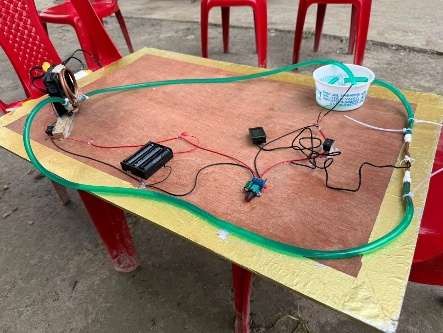
Figure 1: Liquid Cooling System project setup
Methodology
A wooden board was used as the base of the project setup. On this base, the components were secured in place using glue. The pump was powered through 3 batteries connected in series, controlled by a switch for on / off and a voltage regulator to control the flow rate of the pump. The outlet of the pump led to the heated copper tube, then to the coiled copper tube next to the fan, and then to the inlet of the pump. The same water was recirculated within the pipes, taking heat away from the heated tube to the copper coil for cooling. The voltage regulator connected to the pump was used to obtain the 3 types of fluid flow- laminar, transitional and turbulent for 3 different scenarios to compare the cooling rate of the heated tube.
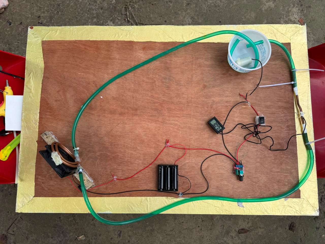
Figure 2: Labelled diagram of the setup
- The pump was turned off and the copper tube to be cooled was heated to a high temperature. The time required for the heated copper tube to reach room temperature was recorded with no circulating water. Thus, the rate of cooling without the pump was determined.
- The pipe for inlet of the pump (inlet here refers to the pipe end that is connected to the inlet of the pump when the cooling system is turned on) was temporarily directed into a 500 mL bottle instead of the inlet.
- The flow rate was determined by dividing the volume of the bottle by the time required to fill it at the specific voltage of the pump. The type of flow was identified to be laminar for the first case.
- The outlet was connected to the inlet of the pump instead of the bottle. The tube was heated again to a high temperature. The time required for the heated tube to reach a low temperature close to the ambient temperature was recorded, and the cooling rate was calculated.
- The voltage regulator value was increased, and steps 2-4 were repeated for the changed voltage for transitional and turbulent flows.
- The cooling rates for the 3 types of flows were calculated and compared using standard formulae of Fluid Mechanics.
Data table
| Flow Type | Time to Fill 500
mL (s) |
Flow Rate (L/min) | Reynolds Number | Initial Temperature (°C) | Final Temperature (°C) | Temperature Difference (°C) | Time Taken (min:s) | Cooling Rate (°C/min) |
| Laminar | 53 | 0.566 | 1890 | 47.3 | 31.2 | 16.1 | 2:57 | 5.46 |
| Transitional | 26 | 1.154 | 3855 | 48.8 | 31.6 | 17.2 | 1:45 | 9.83 |
| Turbulent | 15 | 2.000 | 6680 | 50.0 | 35.1 | 14.9 | 0:55 | 16.25 |
Result
Constants:
A = πD²/4 = 3.167 × 10⁻⁵ m²
Without Liquid Cooling (Pump Off):
Cooling rate = (48.0 − 31.9)/8
= 2.01 °C/min
- Laminar Flow:
Q = 0.0005/53 = 9.43 × 10⁻⁶ m³/s = 0.566 L/min Re = (1000 × (Q/A) × 0.00635)/0.001 = 1890
Cooling rate = (47.3 − 31.2)/2.95 = 5.46 °C/min
- Transitional Flow:
Q = 0.0005/26 = 1.923 × 10⁻⁵ m³/s = 1.154 L/min Re = (1000 × (Q/A) × 0.00635)/0.001 = 3855
Cooling rate = (48.8 − 31.6)/1.75 = 9.83 °C/min
- Turbulent Flow:
Q = 0.0005/15 = 3.33 × 10⁻⁵ m³/s = 2.00 L/min Re = (1000 × (Q/A) × 0.00635)/0.001 = 6680
Cooling rate = (50.0 − 35.1)/0.917 = 16.25 °C/min
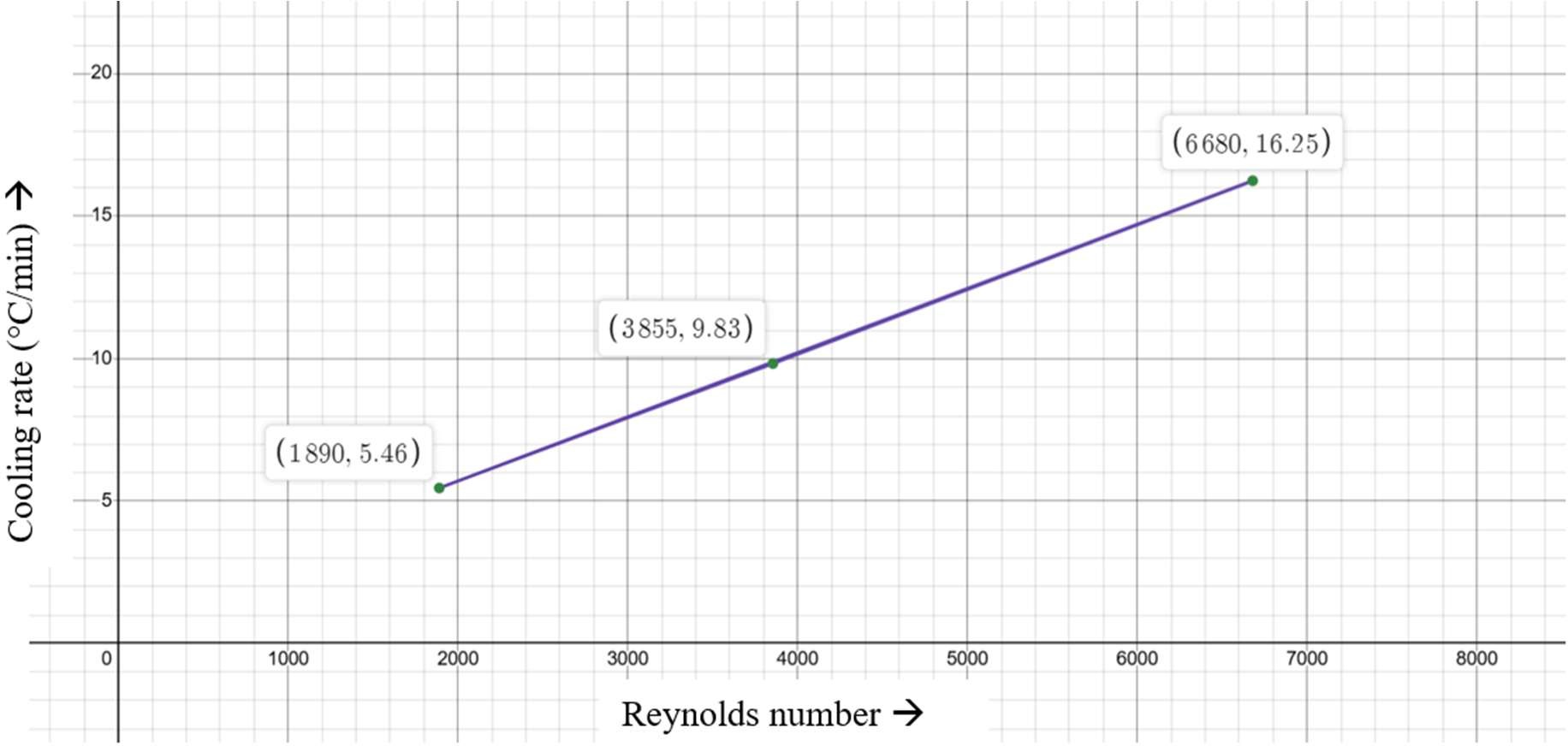
Graph 1: Reynolds number vs Cooling rate
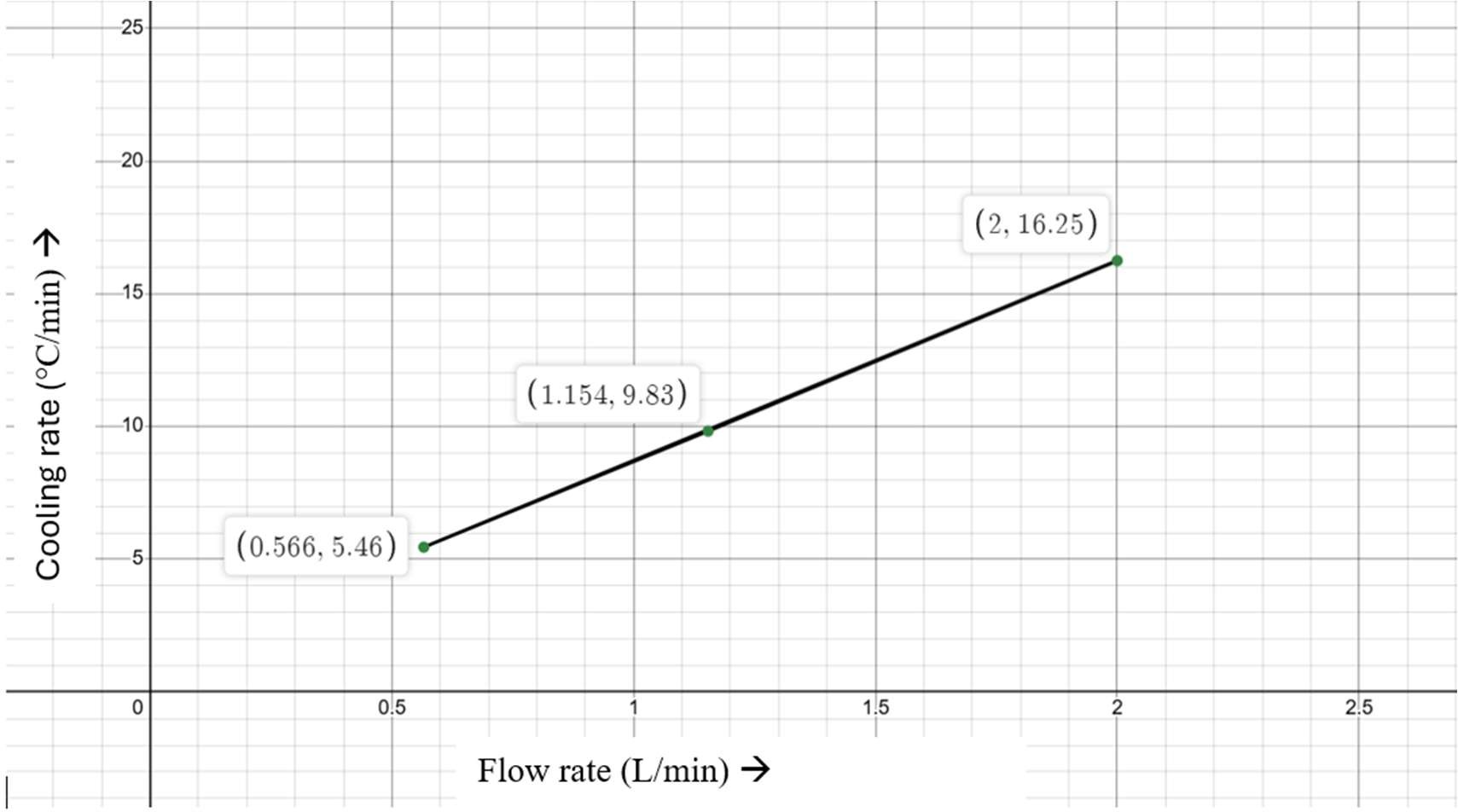
Graph 2: Flow rate vs Cooling rate
From the calculations, it is observed that the cooling rate is higher for turbulent flow compared to transitional and laminar flow. This can be explained by the principles of fluid mechanics. As the Reynolds number reaches the turbulent range for a flowing fluid, there is greater mixing of the flowing fluid, caused by eddies and vortices, whereas for laminar ranges of flow, there is less mixing and lower flow rates. For this experiment,
Re = (ρ× v × D) / μ Where,
Re = Reynolds number ρ = Fluid density
v = Average fluid velocity D = Internal pipe diameter
μ = Dynamic viscosity of the fluid
Since the pipe diameter, density and dynamic viscosity can be considered constant, the only factor that affected the Reynolds number in this experiment was the velocity of the fluid, which was reduced by lowering the regulator knob setting for laminar and increased for turbulent.
The cooling rate for the laminar, transitional and turbulent flows were obtained to be 5.46° C/min, 9.83° C/min and 16.25° C/min respectively, showing an increase in the cooling rate with
increasing Reynolds number. And all these are higher than the cooling rate without the cooling system turned on, which was 2.01 °C/min. The cooling rate for transitional flow was approximately twice that of laminar, and approximately thrice that of laminar in the case of turbulent flow. The higher speed of the fluid caused a greater flow of water at the same time in the heated tube to absorb more of the heat, and since higher velocity also corresponded to higher Reynolds numbers, it caused a more even distribution of the absorbed heat throughout the flowing water.
From the project, it has been shown that the cooling rate changes with Reynolds number, because of faster absorption of heat due to more water flowing through the component to be cooled, and due to better mixing of the fluid at higher Reynolds numbers, causing the heat to spread more evenly. So, it can be concluded that higher Reynolds numbers are better at cooling when it comes to liquid cooling systems.
Uses diverse resources such as equipment, people, software, materials, money, laboratories, and technologies.
| Resources | Project Components |
| Software, computational resources | Desmos |
| Materials | Water, Copper tubes, electronics (pump, motor
controller, switch etc.), transparent pipes, bottles, glue |
| Equipment, Technology | Electronic pump controlled by batteries connected in series |
| Equipment, People | Data acquisition through stopwatch (time taken) and thermometer (temperature changes) |